Combining multiple images

Sometimes users might need to “blend” two or more images. This might be required for showing, for example, the projected stellar density on top of the projected gas density field, or the projected gas density on top of the dark matter distribution.

There are many ways of combining images, and the final result will depend strongly on the adopted algorithm. Py-SPHViewer currently includes only two blending algorithms called “Screen” and “Overlay”. These are included as part of the Blend tools. These blending modes were borrowed from GIMP.

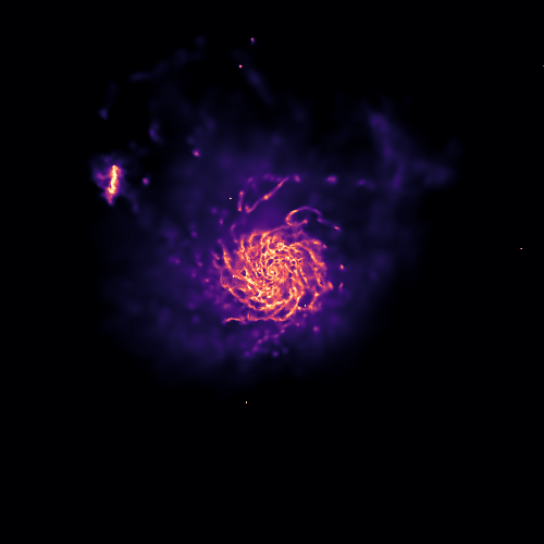
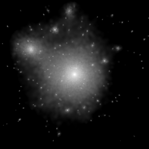
We shall use the individual images shown below, created using the QuickView tool;

Gas distribution

Tutorial about Blending

Dark matter distribution

Tutorial about Blending

Screen blending mode

According the the Screen mode, If $I_{1}$ and $I_{2}$ are RGB images, then the resulting image $I_{f}$ is:

$I_{f} = 255 - \displaystyle\frac{(255 - I_1) \times (255 - I_{2})}{255}$.

This blending mode tends to preserve individual colours relatively well. As explained here, the resulting image is usually brighter. Black regions do not change, and a white regions become fully white in the resulting image. Darker colours in the image appear to be more transparent. The resulting image is independent of the order in which the two images are blended.

We can blend the images using screen as follows:

from sphviewer.tools import Blend
blend = Blend.Blend(rgb_dm,rgb_gas)
output = blend.Screen()

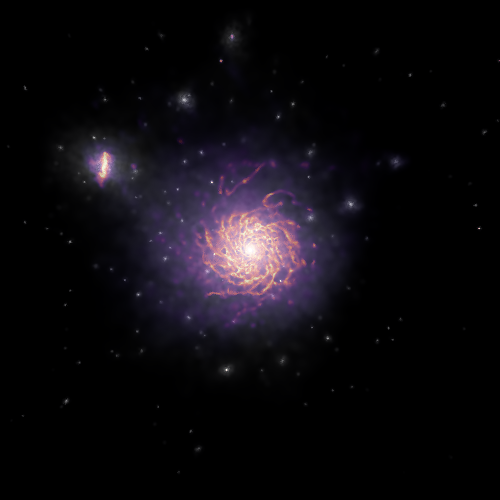
which produces:

Tutorial about Blending

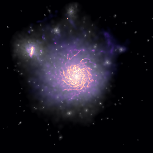
Overlay blending mode

According the the Overlay mode, If $I_{1}$ and $I_{2}$ are RGB images, then the resulting image $I_{f}$ is:

\[I_{f} = \displaystyle\frac{I_{1}}{255} \times \left [ I_{1} + \displaystyle\frac{2I_{2}}{255} \times \left ( 255 - I_{1} \right ) \right ]\]

This blending mode depends on the order in which images are blended. To apply this method we simply call the Overlay method:

from sphviewer.tools import Blend
blend = Blend.Blend(rgb_dm,rgb_gas)
output = blend.Overlay()

which produces:

Tutorial about Blending

For this particular example, the overlay blending mode seems to return the best image.

Finally, blending images may produce very nice results when applied to videos: For example:

import matplotlib as ml
from sphviewer.tools import QuickView, Blend

for p in range(360):    
    cmap_dm = matplotlib.cm.Greys_r
    cmap_gas = matplotlib.cm.magma

    qv_gas   = QuickView(pgas, mass=np.ones(len(pgas)), plot=False, r=200, p=p, t=0)
    qv_drk   = QuickView(pdrk, hsml=hsml, mass=np.ones(len(pdrk)), plot=False,  r=200, p=p, t=0)
    img_gas  = qv_gas.get_image()
    img_drk  = qv_drk.get_image()

    rgb_dm  = ml.Greys_r(get_normalized_image(img_drk, 0, 2.5))
    rgb_gas = ml.magma(get_normalized_image(img_gas, 0.3, 1.7))

    blend = Blend.Blend(rgb_dm, rgb_gas)
    rgb_output = blend.Overlay()

    plt.imsave('snap_%03d.png'%p, rgb_output)

Previous examples creates two different images using QuickView, one for the gas, and for the dark matter. The loop is done over the angle $\phi$ (p), between 0 and 360. Individual images are then converted to RGB images through matplotlib.colors.LinearSegmentedColormap. get_normalized_image is a very simple function that normalizes the image so that we can set the minimum/maximum value below/above which the image saturates:

def get_normalized_image(image, vmin=None, vmax=None):
    if(vmin == None):
        vmin = np.min(image)
    if(vmax == None):
        vmax = np.max(image)

    image = np.clip(image, vmin, vmax)
    image = (image-vmin)/(vmax-vmin)

    return image

The resulting video, after concatenating individual images, is shown below:

Tutorial about Blending