Projections in Py-SPHViewer

Scene Projections

Images in Py-SPHViewer are created by projecting a scene onto a plane, and there are different ways of doing this.

Py-SPHViewer supports two types of projections: parallel and perspective. The key difference between these projections lies in the observer’s position relative to the scene.

• In parallel projection, the observer is placed at infinity, resulting in no perspective distortion.
• In perspective projection, the observer is positioned at a finite distance, introducing perspective effects.

Below, we will demonstrate both projection methods and highlight their differences.

Please download this file before proceeding with the tutorial.

Parallel Projection

As shown in the QuickView tutorial, we can create an image of the dark matter halo with a parallel projection using the following code:

import matplotlib.pyplot as plt
import h5py
from sphviewer.tools import QuickView

qv_parallel = QuickView(pos, r='infinity', plot=False,
                        x=0, y=0, z=0, extent=[-0.1, 0.1, -0.1, 0.1])

hsml = qv_parallel.get_hsml()

fig = plt.figure(1, figsize=(6,6))
imshow(qv_parallel.get_image(), extent=qv_parallel.get_extent(),
       cmap='gist_stern', origin='lower')
plt.show()

This produces the following image:

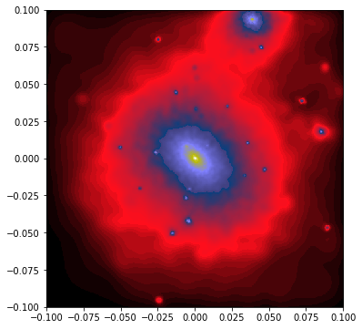
Here, we’ve introduced a few new elements compared to the basic QuickView example. The r='infinity' argument specifies a parallel projection, placing the observer at infinity.

• x=0, y=0, z=0 sets the camera’s target at the center of the dark matter halo.
• extent=[-0.1, 0.1, -0.1, 0.1] defines the field of view, capturing 0.1 Mpc to the left and right of x=0, and 0.1 Mpc above and below y=0.

The qv.get_extent() method returns the actual physical extent of the image. Without this, matplotlib would simply display the pixel count.

Now, let’s modify the parameters to zoom in on a subhalo located at x=0.005 and y=-0.045:

qv_subhalo = QuickView(pos, hsml=hsml, r='infinity', plot=False,
                       x=-0.005, y=-0.045, z=0, extent=[-0.02, 0.02, -0.02, 0.02])

fig = plt.figure(1, figsize=(6,6))
imshow(qv_subhalo.get_image(), extent=qv_subhalo.get_extent(),
       cmap='gist_stern', origin='lower')
plt.show()

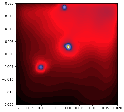
Here, we’ve added the hsml argument, which stores the SPH smoothing lengths of the particles. Py-SPHViewer calculates these lengths in parallel, which can be computationally expensive, so it’s best to reuse them when possible.

Next, let’s explore perspective projection.

Perspective Projection

In perspective projection, objects closer to the camera appear larger, while distant objects appear smaller. This effect is automatically handled when the camera is placed at a finite distance from the scene. By replacing r='infinity' with r=0.1 in the previous example, we position the camera 0.1 Mpc away from the halo:

import matplotlib.pyplot as plt
import h5py
from sphviewer.tools import QuickView

qv_perspective = QuickView(pos, r=0.1, plot=False,
                           x=0, y=0, z=0, extent=[-0.1, 0.1, -0.1, 0.1])

fig = plt.figure(1, figsize=(6,6))
imshow(qv_perspective.get_image(), extent=qv_perspective.get_extent(),
       cmap='gist_stern', origin='lower')
plt.show()

This produces the following image:

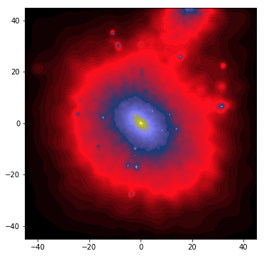
While the two images may look similar, the projection method changes how the scene is rendered. Notice that the image’s limits range from -45 to +45, which now represent the angular size of the scene. The default field of view (FoV) is 90 degrees, though this can be adjusted using the zoom parameter.

The relationship between the camera distance r, magnification M (the zoom variable), and the linear size of the scene l is given by:

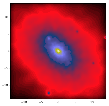
We can zoom in on the inner 0.05 Mpc of the halo by either decreasing r or increasing M. Changing r moves the camera closer, while changing M adjusts the FoV. The latter method retains the current camera position and adjusts the scene’s magnification.

To render the inner 0.05 Mpc at a distance of 0.1 Mpc, we should use M=4 (i.e., FoV ≈ 26°):

qv_perspective = QuickView(pos, r=0.1, plot=False,
                           x=0, y=0, z=0, extent=[-0.1, 0.1, -0.1, 0.1], zoom=4)

fig = plt.figure(1, figsize=(6,6))
imshow(qv_perspective.get_image(), extent=qv_perspective.get_extent(),
       cmap='gist_stern', origin='lower')
plt.show()

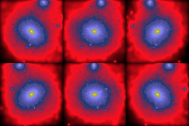
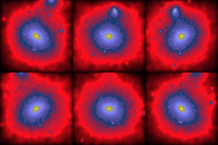
Finally, the images below show a rotation along the vertical axis for both the parallel and perspective projections: