Blending images in PySPHViewer

Combining Multiple Images

Sometimes, users may need to “blend” two or more images. This might be required, for example, to display the projected stellar density on top of the projected gas density field, or the projected gas density on top of the dark matter distribution.

There are many ways to combine images, and the final result depends heavily on the algorithm used. Py-SPHViewer currently includes two blending algorithms called Screen and Overlay, which are part of the Blend tools. These blending modes are adapted from GIMP.

We will use the individual images shown below, created using the QuickView tool:

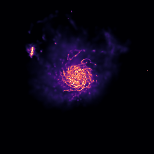
Gas distribution:

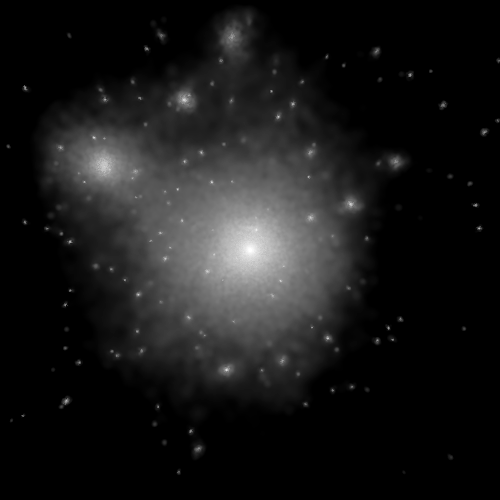
Dark matter distribution:

Screen Blending Mode

According to the Screen mode, if \(I_{1}\) and \(I_{2}\) are RGB images, the resulting image \(I_{f}\) is:

\(I_{f} = 255 - \displaystyle\frac{(255 - I_1) \times (255 - I_{2})}{255}\).

This blending mode tends to preserve individual colors relatively well. As explained here, the resulting image is usually brighter. Black regions remain unchanged, while white regions become fully white in the final image. Darker colors in the image appear more transparent. The resulting image is independent of the order in which the two images are blended.

We can blend the images using Screen as follows:

from sphviewer.tools import Blend
blend = Blend.Blend(rgb_dm, rgb_gas)
output = blend.Screen()

This produces:

Overlay Blending Mode

According to the Overlay mode, if \(I_{1}\) and \(I_{2}\) are RGB images, the resulting image \(I_{f}\) is:

\(I_{f} = \displaystyle\frac{I_{1}}{255} \times \left [ I_{1} + \displaystyle\frac{2I_{2}}{255} \times \left ( 255 - I_{1} \right ) \right ]\).

This blending mode depends on the order in which images are blended. To apply this method, we simply call the Overlay method:

from sphviewer.tools import Blend
blend = Blend.Blend(rgb_dm, rgb_gas)
output = blend.Overlay()

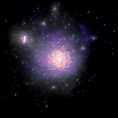
This produces:

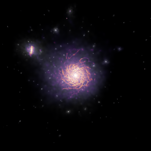
In this particular example, the overlay blending mode seems to return the best result.

Finally, blending images can produce very nice effects when applied to videos. For example:

import matplotlib as ml
from sphviewer.tools import QuickView, Blend

for p in range(360):    
    cmap_dm = matplotlib.cm.Greys_r
    cmap_gas = matplotlib.cm.magma

    qv_gas = QuickView(pgas, mass=np.ones(len(pgas)), plot=False, r=200, p=p, t=0)
    qv_dm = QuickView(pdrk, hsml=hsml, mass=np.ones(len(pdrk)), plot=False, r=200, p=p, t=0)
    img_gas = qv_gas.get_image()
    img_dm = qv_dm.get_image()

    rgb_dm = ml.Greys_r(get_normalized_image(img_dm, 0, 2.5))
    rgb_gas = ml.magma(get_normalized_image(img_gas, 0.3, 1.7))

    blend = Blend.Blend(rgb_dm, rgb_gas)
    rgb_output = blend.Overlay()

    plt.imsave('snap_%03d.png' % p, rgb_output)

The above example creates two different images using QuickView, one for gas and one for dark matter. The loop runs over the angle \(\phi\) (p), ranging from 0 to 360. Individual images are converted to RGB using matplotlib.colors.LinearSegmentedColormap. The function get_normalized_image normalizes the image so that the minimum and maximum values control the saturation:

def get_normalized_image(image, vmin=None, vmax=None):
    if vmin is None:
        vmin = np.min(image)
    if vmax is None:
        vmax = np.max(image)

    image = np.clip(image, vmin, vmax)
    image = (image - vmin) / (vmax - vmin)

    return image

The resulting video, after concatenating individual images, is shown below: